The MPDS application programming interface (API) presents the materials data of the PAULING FILE database online in the machine-readable formats, suitable for automated processing. The intended audience is software engineers and data scientists. The API is available by a subscription (SLA). To start using the API the reader needs a valid API key from the MPDS account. We encourage to contact us for opening such the account.
Some parts of the data are opened and freely available. In particular, these are: (a) cell parameters - temperature diagrams and cell parameters - pressure diagrams, (b) all data for compounds containing both Ag and K, (c) all data for binary compounds of oxygen, (d) all data generated by machine learning, and (e) all data generated by first-principles calculations.
A tech-savvy reader may also explore Jupyter notebooks (also in Binder) and kickoff Python demos. Important: using the API keys within the third-party environment like Binder is potentially insecure and should be done with the greatest care. Should the reader be not familiar with the materials science, just wishing to crunch the data, this quick tutorial can be recommended.
§1. Downloading data
§1.1. MPDS data model
The standard unit of the MPDS data is an entry. All the MPDS entries are subdivided into three kinds: crystalline structures, physical properties, and phase diagrams. They are called S-, P- or C-entries, correspondingly. Entries have persistent identifiers (similar to DOIs), e.g. S377634, P600028, C100026. These identifiers are used in the stable URLs, e.g. https://mpds.io/entry/C100026 and therefore citable, their persistence is guaranteed.
Another dimension of the MPDS data is the distinct phases. The three kinds of entries are interlinked via the distinct materials phases they belong. A tremendous work was done by the PAULING FILE team in the past 20 years to manually distinguish about 200 000 inorganic materials phases, appearing in the literature. Each phase has a unique combination of (a) chemical formula, (b) space group, (c) Pearson symbol. Each phase has the permanent integer identifier called phase_id, also used in the stable citable URLs, such as https://mpds.io/phase_id/7268. An analogous concept is the Materials Project IDs, such as mp-2657, matching the above mentioned MPDS phase_id 7268.
Consider the following example of the entries and distinct phases. There can be the following distinct phases for the titanium dioxide: rutile with the space group 136 (let us say, phase_id 1), anatase with the space group 141 (phase_id 2), and brookite with the space group 61 (phase_id 3). Then the S- and P-entries for the titanium dioxide must refer to either 1, or 2, or 3, and the C-entries must refer to 1, 2, and 3 simultaneously.
Our relatively new development is the machine-learning data generated from the original peer-reviewed data for the less known phases. Such data are always clearly attributed and not supplied by default. So far only the P-entries (10 physical properties) were predicted and thus can be of the machine-learning data type. For some of these properties we also provide our in-house ab initio calculations data, based on the experimental (carefully relaxed) crystalline structures. See below how to enable all these new data types in our API outputs.
Additionally we support the Optimade unified access interface. The Optimade stands for the Open Databases Integration for Materials Design and defines a standardized way for a programmatic access to any online materials database. Please, refer to the Optimade website for the details.
§1.2. Categories of data
The most common task is to get the MPDS data according to some search criteria. We support 14 basic criteria for searching and downloading the entries:
| Facet | Machine-readable name | Examples | Case sensitivity |
|---|---|---|---|
| Physical properties (see the MPDS physical properties hierarchy, numerical properties specifically) |
props | conductivity | no |
| Chemical elements | elements | Cs, Fr-O | no |
| Materials classes (various groups of terms: i.e. mineral names, periodic groups, physical classes, element count keywords etc., see examples) | classes | perovskite, quaternary | no |
| Crystal system | lattices | orthorhombic | no |
| Chemical formula | formulae | SrTiO3, O3Al2, A2B | no |
| Space group (number or international short symbol) | sgs | 221, Pm-3m | no |
| Prototype system ("Strukturbericht" or formula, Pearson symbol, space group number) | protos | D51, SiS2 oI12 72 |
yes |
| Polyhedron atoms (center, ligands) | aeatoms | U, X-Se, UO6, UX7 (X = any atom) |
no |
| Polyhedral type (see all supported types) | aetypes | icosahedron 12-vertex | yes |
| Publication author | authors | Evarestov | no |
| CODEN (code of publication journal, see CODEN index) | codens | PPCPFQ | no |
| Publication years | years | 1960-1990 | — |
| Author location | geos | United Arab Emirates | yes |
| Author organization | orgs | CSIRO | yes |
Thus, in an API request it is possible to combine all these criteria in a reasonable manner. Combination is always done implying conjunctive AND operator. The reasonable manner means one can combine e.g. publication authors with publication years, but cannot combine chemical formulae with chemical elements or space group with crystal system, i.e. the common sense rules in chemistry and physics are implied.
We distinguish the single-term categories, such as the physical properties and crystal systems, and many-term categories, such as the materials classes and publication authors. A combination of terms from the single-term category is not supported. That is, one cannot search for both band gap and conductivity. A combination of terms from the many-term category is easily possible. That is, one can search for both binaries and perovskites.
The single-term categories are props, lattices, formulae, sgs, protos, aeatoms, codens, geos, and orgs. The many-term categories are elements, classes, aetypes, authors, and years.
§1.3. REST-alike download endpoint
To serve data we employ the single REST-alike endpoint, following the HTTP protocol basics. We support input parameters in the query string and request header. We provide the standard HTTP status codes in response. The address of the data download endpoint is the following:
The HTTP verb to be used is always GET. The header must always contain the Key string with the valid MPDS API key, obtained from the corresponding MPDS account. A minimal curl example reads:
The following query string parameters are supported:
| Parameter | Type | Description |
|---|---|---|
| q | JSON-serialized object | The object q may contain any reasonable combination of criteria, given in the Table 1, column "Machine-readable name". Always required. |
| phases | string or integer | Distinct phase identifiers (called phase_id's) separated by commas can be optionally supplied to limit the search. This is convenient for programmatic chained searches one after another. A relevant q parameter must be always given. The count of phase_id's per a single request cannot exceed 1000. |
| dtype | integer | Data type. Possible values: 1 or MPDSDataTypes.PEER_REVIEWED (original data), 2 or MPDSDataTypes.MACHINE_LEARNING (data generated by machine learning), 4 or MPDSDataTypes.AB_INITIO (in-house simulations data), and 7 or MPDSDataTypes.ALL (all mentioned types). Default value: 1 (original data). |
| pagesize | integer | The maximum number of hits per a single response (pagination). Default value: 10. Allowed values: 10, 100, 500, and 1000. |
| page | integer | The page number, either in the selected or in the default pagination. Counts from 0. Defaults to the first page, which has number 0, i.e. the default value is 0. |
| fmt | integer | Output data format. Can be json or cif. The latter cif only makes sense for the crystalline structures. Default value: json. |
An example of the q parameter to request the crystalline structures (with the spaces and line breaks added for readability):
Another example of the q parameter to request the physical properties:
Please, note: we do not support querying by entry IDs in the API intentionally. Although the entry IDs are stable, the entry contents might be updated, changed, or deactivated with time, therefore we advice not to rely on their IDs in the API data mining in the mass manner. Use GUI to get the particular entries by their IDs.
By default the response has json format, containing the following properties: out (list i.e. array of the MPDS entries), npages (number of pages in the selected or default pagination), page (current page number), count (total number of hits), and error (should be null). Some other properties might be added in future.
Each kind of entries (i.e. S- or P-entries) has its own specific properties in JSON (see below).
And if no results are found:
The output in cif format presents nothing more than concatenated CIFs in a plain text.
The response for a correctly understood request will always have the status code 200, whereas the status codes 400 ("Wrong parameters") or 403 ("Forbidden") may signal about an error in the request. Also, 429 ("Too many requests") tells that the request rate should be decreased. Generally, checking the response status code should be always done first.
§1.4. JSON schemata of the MPDS entries
JSON is the first-class-passenger format in the MPDS API. We provide JSON schemata for all kinds of the MPDS entries in the API output. This is visualized below:
Any MPDS API JSON output can be validated against the above schemata e.g. using a Python script below. In the following example the external httplib2 and jsonschema Python packages are used:
#!/usr/bin/env python

import sys
import json
import httplib2
from jsonschema import validate, Draft4Validator
from jsonschema.exceptions import ValidationError

try: input_json = sys.argv[1]
except IndexError: sys.exit("Usage: %s input_json" % sys.argv[0])

network = httplib2.Http()
response, content = network.request("https://developer.mpds.io/mpds.schema.json")
assert response.status == 200

schema = json.loads(content)
Draft4Validator.check_schema(schema)

target = json.loads(open(input_json).read())

if not target.get("npages") or not target.get("out") or target.get("error"):
    sys.exit("Unexpected API response")

try:
    validate(target["out"], schema)
except ValidationError, e:
    raise RuntimeError(
        "The item: \r\n\r\n %s \r\n\r\n has an issue: \r\n\r\n %s" % (
            e.instance, e.context
        )
    )
All the MPDS data without exceptions are expected to be valid against the supplied schemata.
§1.5. Example scripts
Below are simple examples for the MPDS data retrieval in two programming languages: Python and JavaScript. More languages can be added by request. Note, that the Python example requires an external package httplib2. We provide more convenient Python client library, so these examples serve demonstration purposes only.
#!/usr/bin/env python

from urllib.parse import urlencode
import httplib2
import json


api_key = "" # your key
endpoint = "https://api.mpds.io/v0/download/facet"
search = {
    "elements": "Mn",
    "classes": "binary, oxide",
    "props": "isothermal bulk modulus",
    "lattices": "cubic"
}

req = httplib2.Http()
response, content = req.request(
    uri=endpoint + '?' + urlencode({
        'q': json.dumps(search),
        'pagesize': 10,
        'dtype': 2 # see parameters documentation above
    }),
    method='GET',
    headers={'Key': api_key}
)

if response.status != 200:
    # NB 400 means wrong input, 403 means authorization issue etc.
    # see https://en.wikipedia.org/wiki/List_of_HTTP_status_codes
    raise RuntimeError("Error code %s" % response.status)

content = json.loads(content)

if content.get('error'): raise RuntimeError(content['error'])

print("OK, got %s hits" % len(content['out']))
#!/usr/bin/env node

var https = require('https');
var qs = require('querystring');

var api_key = ""; // your key
var host = "api.mpds.io", port = 443, path = "/v0/download/facet";
var search = {
    "elements": "Mn",
    "classes": "binary, oxide",
    "props": "isothermal bulk modulus",
    "lattices": "cubic"
};

https.request({
    host: host,
    port: port,
    path: path + '?' + qs.stringify({q: JSON.stringify(search), pagesize: 10, dtype: 2}),
    method: 'GET',
    headers: {'Key': api_key}
}, function(response){
    var result = '';
    if (response.statusCode != 200){
        // NB 400 means wrong input, 403 means authorization issue etc.
        // see https://en.wikipedia.org/wiki/List_of_HTTP_status_codes
        return console.error('Error code: ' + response.statusCode);
    }
    response.on('data', function(chunk){
        result += chunk;
    });
    response.on('end', function(){
        result = JSON.parse(result);
        if (result.error) console.error(result.error);
        else {
            console.log('OK, got ' + result.out.length + ' hits');
        }
    });
}).on('error', function(err){
    console.error('Network error: ' + err);
}).end();
§1.6. API and GUI
The MPDS data provided in API and GUI (graphical user interface) are generally the same. There are however two important points to consider.
First, the GUI is intended for the human researchers, not for the automated processing. Therefore the data in GUI are less rigorously formatted, being thus closer to the original publications (which, of course, impedes machine analysis).
Second, some portion of data (~15%) present in the GUI is absent in the API. This is because currently a number of MPDS entries has only textual content or even no content at all (in process of preparation), i.e. present little value for the data mining. However, we make our best to expose the maximum MPDS data in the API, and this is the work in progress.
To summarize, the API differs from GUI in the following: (a) machine-readable (and to a certain extent machine-understandable), (b) programmer-friendly, pluggable and integration-ready, (c) massively exposing the data, i.e. all the MPDS content can be analyzed in minutes. Thus, thanks to the API, the MPDS platform can be used in variety of the other scientific ways, which we had never designed. So the researchers get unprecedented flexibility and power, which is unthinkable within the GUI.
§2. Processing data
§2.1. Overview
To facilitate starting with the MPDS API we provide several exercises (or miniature case studies): (a) distribution density analysis, (b) clustering, and (c) correlation search. To a certain extent they could be considered as recipes, however aiming to illustrate the informatics aspect, not the materials science aspect. All these exercises are described below and can be found in the Github repository.
There is also a number of Jupyter notebooks: (a) basic plotting using the periodic table, (b) machine-learning and peer-reviewed data, (c) unusual materials phases from the machine learning, (d) pVT-data and EoS fitting. They can be launched online from GitHub using e.g. Binder environment.
The reader now may decide, whether to follow a text with the code listings below ("classical way"), or to download and run the Python scripts ("Python way"), or play with the Jupyter notebooks interactively online ("ultra-modern way"). Important: using the API keys within the third-party Jupyter environment is potentially insecure and should be done with the great care (see notebooks).
§2.2. Client library
As mentioned, any programming language, able to execute HTTP requests and handle the JSON output, can be employed. However, one of the most frequently used languages in data processing is Python. Therefore we provide a client library for Python. This library takes care of many aspects of the MPDS API, such as pagination, error handling, validation, proper data extraction and more. We encourage our users to adopt this library for their needs. It is installed as any other Python library:
The exercises below use this library. Some of them might also employ numpy, scipy, and pandas libraries (a popular data science toolbox). As a necessary preparation, we save the MPDS API key in an environment of our terminal session. Later the Python API client reads the key from there, if not explicitly provided. For Bash:
Note, that there are three fundamental data types at the MPDS concerning the data origin: peer-reviewed, in-house machine-learning, and in-house first-principles simulations. By default only the peer-reviewed data are always supplied in the API. To change this using the Python library, one has to setup the dtype attribute in advance. As seen below, at first all the data types are enabled, then only the machine-learning type is enabled:
The data type is set up by a client with the dtype query string parameter.
§2.3. Bond length analysis
Let us say we want to study the chemical bond of A and B elements, e.g. uranium and oxygen. What is the length or lengths of this bond the most frequently reported in the world scientific literature? MPDS contains more than 2500 crystalline structures with uranium and oxygen, so why should not we perform a quick data investigation to answer this question. Starting with the necessary imports in Python:
#!/usr/bin/env python
import pandas as pd
from mpds_client import MPDSDataRetrieval
We use a naive brute-force approach to calculate bond lengths between particular atom types in a crystalline environment. Obviously, we are interested in neighboring atoms only, so we do not consider interatomic distances more than, let us say, 4 Å. We then represent a crystalline structure with the ase's Atoms class and calculate distances using its get_distance method. Note rounding of distances marked by comment NB in the code:
def calculate_lengths(ase_obj, elA, elB, limit=4):
    assert elA != elB
    lengths = []
    for n, atom in enumerate(ase_obj):
        if atom.symbol == elA:
            for m, neighbor in enumerate(ase_obj):
                if neighbor.symbol == elB:
                    dist = round(ase_obj.get_distance(n, m), 2) # NB occurrence <-> rounding
                    if dist < limit:
                        lengths.append(dist)
    return lengths
Note that the crystalline structures are not retrieved from MPDS by default, so we need to specify additional four fields: cell_abc, sg_n, basis_noneq, els_noneq. On top of that, we also ask for the phase_id's, MPDS entry numbers, and chemical formulae. Note that get_data API client method returns a usual Python list, whereas get_dataframe API client method returns a Pandas dataframe. We use the former below:
client = MPDSDataRetrieval()

answer = client.get_data(
    {"elements": "U-O", "props": "atomic structure"},
    fields={'S':[
            'phase_id',
            'entry',
            'chemical_formula',
            'cell_abc',
            'sg_n',
            'basis_noneq',
            'els_noneq'
            ]}
)
The MPDSDataRetrieval.compile_crystal API client method helps us to handle the crystalline structure in the ase's Atoms flavor. A popular Pymatgen library can be also used instead. Mind however that these two libraries are generally incompatible, so never mix crystalline structures in ase and Pymatgen flavors.
We then call the calculate_lengths function defined earlier:
lengths = []

for item in answer:
    crystal = MPDSDataRetrieval.compile_crystal(item, 'ase')
    if not crystal: continue
    lengths.extend( calculate_lengths(crystal, 'U', 'O') )
That runs a little bit slow (about five minutes), since ase's Atoms are expectedly not performing very well on dozens of thousands of bond length calculations. We may want to either use the ase's neighbor_list method, or employ a C-extension, but this is outside the scope of this exercise. Anyway now we have a flat list lengths. Let's convert it into a Pandas Dataframe and find which U-O distances occur more often than the others.
dfrm = pd.DataFrame(sorted(lengths), columns=['length'])
dfrm['occurrence'] = dfrm.groupby('length')['length'].transform('count')
dfrm.drop_duplicates('length', inplace=True)
What did we do here? We calculated the numbers of occurrences (counts) of each particular U-O length and then augmented our dataframe with this new information, creating a new column occurrence. (The reader remembers that we have rounded the interatomic distances calculated.)
Now it's up to the reader to visualize the result (this is absolutely a matter of taste). Below is a bar chart rendered using Plotly and D3 JavaScript libraries. We provide visualization exporting toolbox in Python, allowing the export of the results into CSV and JSON formats and reproducing the figures, although its usage is optional.
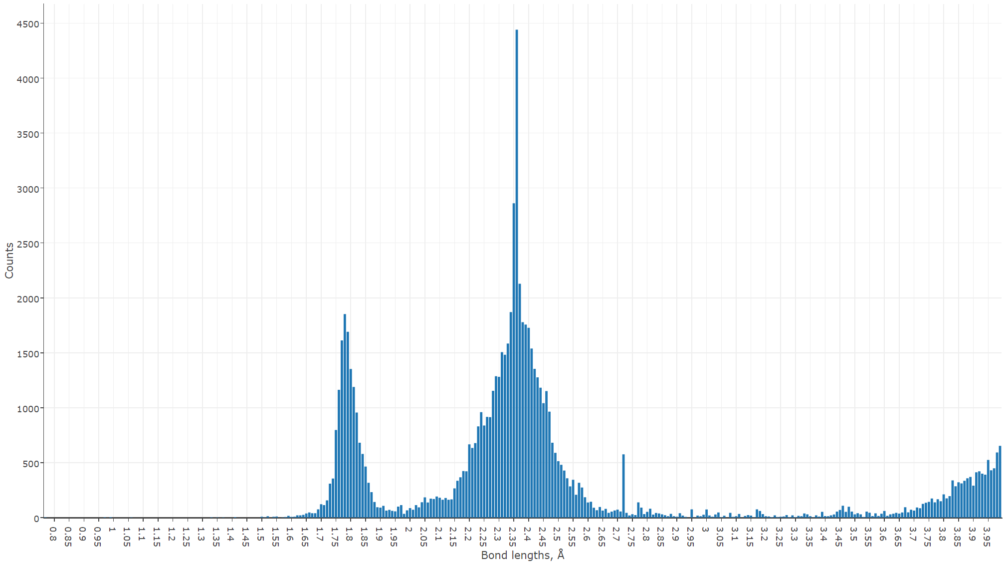
We can see now that the most frequent bond lengths between the neighboring uranium and oxygen atoms are 1.78 and 2.35 Å. This excellently agrees with the well-known study of Burns et al., done in 1997. However, Burns considered only 105 structures, and we did more than 2500, confirming very well although his findings on the uranyl ion geometry.
§2.4. Clustering the band gaps
Unsupervised grouping the values into the clusters in a many-dimensional space is a classical mathematical problem. In an applied data science it is successfully managed using e.g. such algorithms as k-means and Gaussian mixtures.
Taking the non-conducting binary compounds, let us find the clusters in their band gaps and the periodic groups of their elements. That is, we obtain the band gaps and corresponding pairs of the chemical elements, forming a binary compound, and then, for the series of values group of the first element — group of the second element — band gap we apply k-means. Given a set of points (in our case, in a three-dimensional space), k-means aims to partition the points into a number of sets, in order to minimize the within-cluster sum of distance functions of each point to the cluster center.
Here we explicitly specify some fields of P-entries we are interested in. As said, all the fields are given in the JSON schema. Filtering by the units (eV), we get rid of some band gap derivatives, which are also present in the output. Then we remove a couple of unphysical values (negative or more than 20 eV) that are probably wrongly reported:
#!/usr/bin/env python
from ase.data import chemical_symbols
from retrieve_MPDS import MPDSDataRetrieval
from kmeans import Point, kmeans, k_from_n # standalone K-means implementation

client = MPDSDataRetrieval()

dfrm = client.get_dataframe(
    {"classes": "binary", "props": "band gap"},
    fields={'P': [
        'sample.material.chemical_formula',
        'sample.material.chemical_elements',
        'sample.material.condition[0].scalar[0].value',
        'sample.measurement[0].property.units',
        'sample.measurement[0].property.scalar'
    ]},
    columns=['Formula', 'Elements', 'SG', 'Units', 'Bandgap']
)
dfrm = dfrm[dfrm['Units'] == 'eV']
dfrm = dfrm[(dfrm['Bandgap'] > 0) & (dfrm['Bandgap'] < 20)]
Note, that there might be different values of the band gaps reported in the literature for each particular compound. Clearly, this is because we have not specified the character of the desired values (direct or indirect band gap), but even apart of that variations are expected, e.g. due to slightly different experimental conditions. Here we simply take the average of all the values per a compound, although there are of course better ways to handle that:
avgbgfrm = dfrm.groupby('Formula')['Bandgap'].mean().to_frame().reset_index() \
    .rename(columns={'Bandgap': 'AvgBandgap'})
dfrm = dfrm.merge(avgbgfrm, how='outer', on='Formula')
dfrm.drop_duplicates('Formula', inplace=True)
We now have a lot of different binary compounds with the averaged values of band gap. So our data are ready for clustering. This is how we get the periodic element groups:
def get_element_group(el_num):
    if el_num == 1: return 1
    elif el_num == 2: return 18

    elif 2 < el_num < 19:
        if (el_num - 2) % 8 == 0: return 18
        elif (el_num - 2) % 8 <= 2: return (el_num - 2) % 8
        else: return 10 + (el_num - 2) % 8

    elif 18 < el_num < 55:
        if (el_num - 18) % 18 == 0: return 18
        else: return (el_num - 18) % 18

    if 56 < el_num < 72: return 3 # custom group for lanthanoids
    elif 88 < el_num < 104: return 3 # custom group for actinoids
    elif (el_num - 54) % 32 == 0: return 18
    elif (el_num - 54) % 32 >= 17: return (el_num - 54) % 32 - 14
    else: return (el_num - 54) % 32
And this is how we define the points for clustering based on our data:
fitdata = []

for n, row in dfrm.iterrows():
    groupA, groupB = \
        get_element_group(chemical_symbols.index(row['Elements'][0])), \
        get_element_group(chemical_symbols.index(row['Elements'][1]))
    fitdata.append(
        Point(
            sorted([groupA, groupB]) + [round(row['AvgBandgap'], 2)],
            reference=row['Formula']
        )
    )
clusters = kmeans(fitdata, k_from_n(len(fitdata)))
We use a standalone k-means Python implementation kmeans, although the reader might want to employ sklearn or scipy. Note, that the k-means algorithm does not provide the number of clusters to divide our data. We try to guess this number from the size of our data naively using k_from_n function. For homogeneous data this guess is likely to be wrong, but for heterogeneous data it should make sense.
We then export the data in a flat Python list for plotting as follows. The plot below is prepared using the visualization exporting toolbox.
export_data = []

for cluster_n, cluster in enumerate(clusters, start=1):
    for pnt in cluster.points:
        export_data.append(pnt.coords + [pnt.reference] + [cluster_n])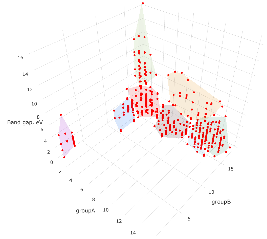
§2.5. Structure-property correlations
In this excercise we quantitatively estimate the relationship between a physical property of interest and the atomic structure. This is the very basic task in chemoinformatics, called QSAR/QSPR study, which stands for the quantitative structure-activity or structure-property relationship modeling. Technically, we request some physical property from MPDS and try to figure out, whether it depends on the crystalline structure, and if yes, how much.
Here the question "how much" is answered by a correlation coefficient, which can be defined either as a measure of how well two datasets fit on a straight line (Pearson coefficient), or difference between concordant and discordant pairs among all the possible pairs in two datasets (Kendall's tau coefficient). Both Pearson and Kendall's tau correlation coefficients are defined between -1 and +1, with 0 implying no correlation. For the Pearson coefficient, values of -1 or +1 imply an exact linear relationship. Positive correlations imply that as x increases, so does y. Negative correlations imply that as x increases, y decreases. For the Kendall's tau coefficient, values close to +1 indicate strong agreement, values close to -1 indicate strong disagreement. Calculation of both these correlation coefficients is provided by pandas Python library.
As usual, we start with the Python imports:
#!/usr/bin/env python
from __future__ import division

import numpy as np
import pandas as pd
from ase.data import chemical_symbols, covalent_radii

from retrieve_MPDS import MPDSDataRetrieval
We then present two descriptors for the crystalline structures. The term descriptor stands for the compact information-rich number, allowing the convenient mathematical treatment of the encoded complex data (crystalline structure, in our case). We employ an APF descriptor, as well as topological Wiener index, defined per a unit cell. It is up to the reader to check the other descriptors for the crystalline structures.
def get_APF(ase_obj):
    volume = 0.0
    for atom in ase_obj:
        volume += 4/3 * np.pi * covalent_radii[chemical_symbols.index(atom.symbol)]**3
    return volume/abs(np.linalg.det(ase_obj.cell))

def get_Wiener(ase_obj):
    return np.sum(ase_obj.get_all_distances()) * 0.5
Note that our descriptors generally depend on whether we use compile_crystal(item, 'ase') or compile_crystal(item, 'pmg'). This is because by default ase and Pymatgen libraries handle crystalline structures in a slightly different manner. The reader is welcomed to edit the code above for the Pymatgen library.
Concerning the property being investigated, we restrict ourselves with some materials classes, in order to reduce the time needed for descriptor calculations:
client = MPDSDataRetrieval()

dfrm = client.get_dataframe({
    "classes": "transitional, oxide",
    "props": "isothermal bulk modulus"
})
dfrm = dfrm[np.isfinite(dfrm['Phase'])]
dfrm = dfrm[dfrm['Units'] == 'GPa'] # cleaning
dfrm = dfrm[dfrm['Value'] > 0] # cleaning

phases = set(dfrm['Phase'].tolist())
answer = client.get_data(
    {"props": "atomic structure"},
    phases=phases,
    fields={'S':[
            'phase_id',
            'entry',
            'chemical_formula',
            'cell_abc',
            'sg_n',
            'basis_noneq',
            'els_noneq'
            ]}
)
descriptors = []

for item in answer:
    crystal = MPDSDataRetrieval.compile_crystal(item, 'ase')
    if not crystal: continue
    descriptors.append(( item[0], get_APF(crystal), get_Wiener(crystal) ))

descriptors = pd.DataFrame(descriptors, columns=['Phase', 'APF', 'Wiener'])
Now we have got the physical property values in the dfrm dataframe and the structure descriptors in the descriptors dataframe. The reader remembers that in MPDS the physical properties and crystalline structures are related via the distinct phase concept, i.e. the same phase identifiers, which we have saved in advance in the Phase columns of dfrm and descriptors dataframes. As the MPDS might have several crystalline structures per a physical property value (or vice versa), we take an average (mean) of all the respective quantities within a distinct phase. After that we join our dataframes using the Phase column:
d1 = descriptors.groupby('Phase')['APF'].mean().to_frame().reset_index()
d2 = descriptors.groupby('Phase')['Wiener'].mean().to_frame().reset_index()
dfrm = dfrm.groupby('Phase')['Value'].mean().to_frame().reset_index()

dfrm = dfrm.merge(d1, how='outer', on='Phase')
dfrm = dfrm.merge(d2, how='outer', on='Phase')

dfrm.drop('Phase', axis=1, inplace=True)
dfrm.rename(columns={'Value': 'Prop'}, inplace=True)
And this is how the both correlation coefficients are calculated:
corr_pearson = dfrm.corr(method='pearson')
corr_kendall = dfrm.corr(method='kendall')

print("Pearson. Prop vs. APF = \t%s" % corr_pearson.loc['Prop']['APF'])
print("Pearson. Prop vs. Wiener = \t%s" % corr_pearson.loc['Prop']['Wiener'])
print("Kendall Tau. Prop vs. APF = \t%s" % corr_kendall.loc['Prop']['APF'])
print("Kendall Tau. Prop vs. Wiener = \t%s" % corr_kendall.loc['Prop']['Wiener'])
Expectedly, we can see some correlation between the selected property (namely, isothermal bulk modulus for the oxides of transitional elements) and two structural descriptors. However it varies considerably with the different materials classes, since the crystalline structure also changes considerably. Using the intuition, may the reader suggest the physical property showing higher correlation with either of two structural descriptors within a certain materials class — or no correlation at all?
§2.6. Visualizations
Although the reader is encouraged to visualize the data using his habitual tools, we provide a set of helper utilities. Using a simple exporting toolbox in our Python client library each of the exercises considered above may output two files for the further plotting: CSV and JSON.
By default these two files are written in a system-wide temporary directory /tmp (subdirectory _MPDS). CSV is commonly used in the electronic sheets (such as OpenOffice Calc), and JSON has a custom self-explanatory layout suitable for the Vis-à-vis web-viewer. This is a browser-based JavaScript application, heavily used inside the MPDS GUI. It employs Plotly and D3 visualization libraries. All JSON produced with the exporting toolbox may be simply drag-n-dropped in the browser window with the loaded Vis-à-vis.
We thank the reader for the time and interest! Any questions or feedback is very welcomed and greatly appreciated.